The model of monopoly
 Monopoly, as a market form, is at the opposite end of the spectrum to perfect competition. In the literal sense, a monopoly exists when one single firm or a small group of firms acting together controls the entire market supply of a good or service for which there are no close substitutes. This is a situation of pure monopoly, which like the case of perfect competition, is rarely easy to identify in reality. Moreover, whether an industry can be classed as a monopoly will depend on how narrowly the industry is defined; for example, a city underground system (metro/subway) often has a monopoly on the supply of underground travel within the city, but does not have a monopoly on all forms of public transport within the city: people can also travel by bus, tram or overground trains.
Thus, in practice, less stringent definitions than 'single producer' tend to be used and economists focus instead on the degree of monopoly power which exists rather than absolute monopoly power. A firm, in the UK, may be regarded as being a monopolist if it controls 25 per cent or more of the total market supply of a particular good or service.
A market concentration ratio is used to measure the degree of concentration within a particular industry or group of industries. A commonly used ratio is the five firm concentration ratio that indicates the proportion of the industry's output produced by the five largest firms.
Theory of monopoly
The monopolist's demand curve
In our analysis of perfect competition, we showed how there is a distinction between the demand curve of the individual firm and that of the market as a whole - the existence of many firms each competing against each other means that each one has no influence over price, and has to take the price that is determined in the market through the intersection of the demand and supply curves. The demand curve for each firm is therefore horizontal: an infinite amount is demanded at one price, with nothing at all being demanded at a higher price and with the charging of a lower price being inconsistent with the goal of profit maximisation.
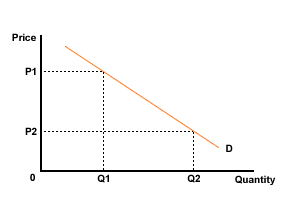
However, under monopoly there is only one firm in the industry; thus there is no difference between the demand curve for the industryand the demand curve for the firm. As the monopolist is subject to the normal law of demand, the monopolist's demand curve will be downward sloping so that to sell more, price would have to be lowered (see figure 1). In comparison to other types of market, the monopolist's demand curve is likely to be relatively inelastic as close substitutes may not be available if price is raised. Indeed, the availability or non-availability of close substitutes is one of the key factors determining the monopolist's power in the market.

Figure 1 Monopolist's demand curve
The demand curve shown in Figure 1 presents the monopolist with a choice. The monopolist can either choose to make the price or the quantity, but cannot do both; for example, if the monopolist chooses to set a price of OP1, the market dictates that only a quantity of OQ1 could be sold; however, if the monopolist chooses to set a quantity of OQ2 to be sold, clearly the demand curve tells us that this could only be achieved at a price of OP2.
Marginal revenue and average revenue under monopoly

The table below assumes that the monopolist faces a normal demand schedule, and from this the revenue curves are derived. Try calculating the figures for total, average and marginal revenue and once you have had a go, follow the link to check your answers.
| Output | Price | Total revenue | Marginal revenue | Average revenue |
|---|---|---|---|---|
| 1 | 20 | |||
| 2 | 18 | |||
| 3 | 16 | |||
| 4 | 14 |
Total, average and marginal revenue answers
From the table two points can be seen:
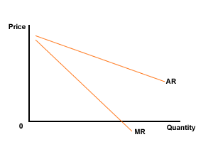
a) As price has to be lowered to increase sales, marginal revenue is not equal to price as in perfect competition: the additional revenue gained from each extra sale is always less than price or average revenue, and thus the MR curve will always be below the AR curve in monopoly.
b) As price is identical to average revenue, the demand curve is also the curve relating average revenue to the quantity produced.
The information in this table can now be shown in diagrammatic form to show the relationship between the average and marginal revenue curves (figure 2).

Figure 2 Marginal and average revenue curves
