Microeconomics

Table of Contents

1. Topic pack - Microeconomics - introduction
2. 1.1 Competitive Markets: Demand and Supply
3. 1.1 Competitive Markets: Demand and Supply - notes
4. 1.1 Competitive markets - questions
5. 1.1 Competitive markets - simulations and activities
6. 1.2 Elasticities
7. 1.2 Elasticities - notes
8. Section 1.2 Elasticities - questions
9. Section 1.2 Elasticities - simulations and activities
10. 1.3 Government intervention
11. 1.3 Government Intervention - notes
12. 1.3 Government intervention - questions
13. 1.3 Government intervention - simulations and activities
14. 1.4 Market failure
15. 1.4 Market failure - notes
16. Section 1.4 Market failure - questions
17. Section 1.4 Market failure - simulations and activities
18. 1.5 Theory of the firm
19. 1.5 Theory of the firm - notes (HL only)
    1. Cost theory
    2. Calculating costs
    3. Short-run
    4. Long-run
    5. Internal economies of scale
    6. External economies of scale
    7. Diseconomies of scale
    8. Long run cost curves
    9. The very long run
    10. Revenues
    11. Revenues - notes
    12. Profit
    13. Profit - notes
    14. Combining revenue and cost curves
    15. Profit maximisation - price taker
    16. Profit maximisation - price setter
    17. Alternative aims of firms
    18. Profit, sales and revenue maximisation
    19. Perfect competition
    20. Perfect competition - notes
    21. Short-run to long-run - profits
    22. Short-run to long-run - losses
    23. Shut down price, break-even price
    24. Efficient allocation of resources
    25. Monopoly and oligopoly
    26. Monopoly and oligopoly - introduction
    27. Growth and power
    28. The model of monopoly
    29. Monopoly - profit maximisation
    30. Monopoly equilibrium
    31. Monopoly v. perfect competition
    32. Economic efficiency in perfect competition
    33. Economic efficiency in perfect competition and monopoly
    34. Efficiency and market structure
    35. Monopolistic competition
    36. Monopolistic competition - notes
    37. Monopolistic competition in the short-run
    38. Monopolistic competition in the long run
    39. Oligopoly
    40. Oligopoly - notes
    41. Advertising and branding
    42. Product innovation
    43. Theories of oligopoly - non-collusive
    44. The kinked demand curve theory
    45. Kinked demand curve - change in cost
    46. Cut-price competition (predatory pricing)
    47. Theories of oligopoly - collusive
    48. Forms of collusion
    49. Price discrimination
    50. Equilibrium of the discriminating monopolist
20. Section 1.5 Theory of the firm - questions
21. Section 1.5 Theory of the firm - simulations and activities
22. Print View

Calculating costs

You also need to be able to calculate a firm's costs from given data, be able to draw cost curves and then interpret what they mean. We come to that skill later.

You will also need to identify and explain short-run and long-run cost curves. Look carefully at the following examples.

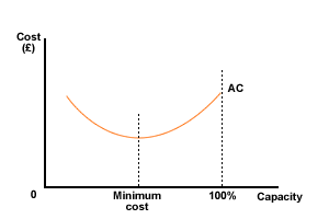
Figure 3 Short-run average cost curve

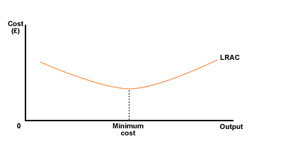
Figure 4 Long-run average cost curve

In the short-run, at least one factor input is fixed. In the long-run all inputs are variable. This means that short-run curves are models of what is happening. Long-run curves are planning data. A firm cannot operate with all inputs variable. Having decided what it wants from an examination of the long-run curves, the firm makes a decision to fix a factor, usually capital, and this gives rise to a new short-run situation.

Now, the calculations and the drawing!

You could be presented with data in the form of a table, like the one below

Plot this with output on the horizontal axis and total cost on the vertical axis and look at it.

There is also a static version of this graph available.

What do you know now?

• The firm has fixed costs of $100,000, the cost of 'output zero'.
• The total variable cost is increasing with increasing output

Now, some more sums. Work out the average cost (TC / output), the total variable cost (TC - FC), the variable cost (TVC / output), the average fixed cost (FC / Output) and the marginal cost (TC (Qx) - TC (Qx-1)).

Once you have had a go at calculating all these, follow the answer link below to compare how you got on.

Answer - cost calculations

Now plot this data on two separate graphs as follows, and see what it shows.

Graph 1 - Total cost, total variable costs and total fixed costs
Graph 2 - Marginal cost, average cost, average fixed cost and average variable cost

You should get the following:

Graph 1 Total cost, total variable costs and total fixed costs

There is also a static version of this graph available.

Graph 2 - Marginal cost, average cost, average fixed cost and average variable cost

There is also a static version of this graph available.

• Average cost (AC) falls initially, then turns and starts to rise.
• AFC + AVC = AC.
• MC follows the same pattern, but at a more exaggerated rate.
• Marginal cost and average cost cross at the minimum average cost.

See Figure 6 below for the standard representation of these curves.

Why do average and marginal cost cross at the minimum point of average cost?

Well think of this in terms of cricket scores. Your last innings is your 'marginal' innings, whereas your batting average is your 'average'. Say your average is 50 and in your next innings you get 20 runs. What happens to your average? It will fall. However, if in your next innings you get 80 runs. In this case your average will rise.

So, if the marginal is below the average, the average will fall and if the marginal is above the average, the average will rise.

There are many questions for you to work on in the questions section (click on the questions - module 2 link in the left hand navigation bar). It may also be worth having a look at the Diggin' diagrams sections (accessible from the course homepage) to check how well you understand your diagrams.

Summary

Remember, a standard marginal and average cost curve diagram should look like this:

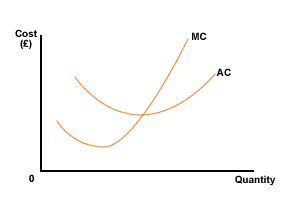
Figure 5 Marginal and average cost

Add in the average fixed and average variable cost curves and it should look like this:

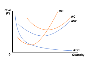
Figure 6 Marginal cost, average cost, average fixed cost and average variable cost