Short-run

It is important to know the difference between the short run and the long run. The law of diminishing returns is a short run law. Economies and diseconomies of scale occur in the long run.

$S:\TripleA\Design\icons\small\key_terms.gif$

Short run

The short run is the period of time in which at least one factor of production is fixed. Over this time period the firm can only expand production by using more of the variable factor.

$S:\TripleA\Design\icons\small\key_terms.gif$

Long run

The long run is the period of time when all factor inputs, including capital, can be changed.

You need to remember these as the time period makes a big difference to how the firm can react to changes in circumstances. In the short-run their capacity is fixed and so all they can do is employ more variable factors. They cannot expand the scale or size of the firm. In the long-run though they can. We put the word scale in bold just now because it is important - economies of scale will only arise in the long-run. In the short-run we get diminishing returns to a factor (because the firm can only change the variable factor).

If you would prefer to view this interaction in a new web window, then please follow the link below:

Law of diminishing returns

This theory supports the shape of the marginal and average cost curves. Both of these curves will be u-shaped as eventually diminishing returns will lead to costs increasing. Initially increasing returns mean that both AC and MC will fall, but once diminishing returns set in both curves start to rise again. The MC and AC curves are shown in Figures 2 and 3, although we will return to these in more detail in the next section.

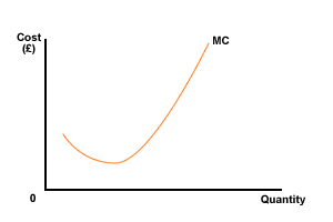
Figure 2 Marginal cost curve

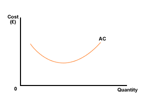
Figure 3 Average cost curve

The marginal cost curve will intersect the average cost curve at its minimum point.

The actual position of the AC curve will vary with a number of factors.

Costs of factor inputs (labour, materials, services etc). The cheaper the inputs the lower the average cost will be at any given output.
Productivity - productivity can be defined as output per unit input. The more productive the firm, the more output it gets from its inputs and the lower the average cost at any output.

Productivity is measured in a number of ways:

Marginal product (MP) - the change in total output resulting from the adding of one extra unit of a variable factor, often labour.
Average product (AP) - total output / units of variable factor being used.

The choice of factor inputs will be driven by their costs, productivity and effect on product cost. An efficient firm will make its choices so as to minimise its average cost at the production rate being worked. Look at the following example.

Example

Student Computers make DVD drives. Its average cost curve is shown in figure 4 below.

ac_ex1

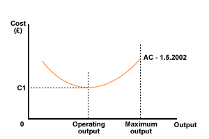
Figure 4 Average cost curve for Student Computers on 1^st May 2002

The following then takes place:

Business rates increase (fixed costs (FC))
Insurance premiums rise (FC)
Wage rates (variable costs (VC)) and salaries (FC) increase

This will change the cost curves. The curve will move upwards due to the increase in fixed costs. The average cost of production at the present output will rise from C1 to C2. Unless something is done about it, the profits will fall.

ac_ex2

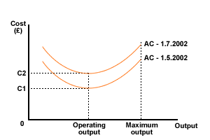
Figure 5 Average cost curves for Student Computers on date 1

In response to these changes the research and development department introduces new materials that are cheaper to buy than the old ones. They also introduce new working practices and procedures that increase productivity considerably. The savings are shared between the firm and its employees. This all reduces variable costs and the AC curve falls again. Now the production average cost, at C3, is lower than before.

ac_ex3

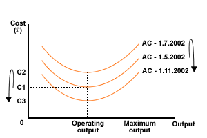
Figure 6 Average cost curves for Student Computers on date 2

The firm has responded to rises in certain costs by taking steps to reduce others.

Microeconomics

Table of Contents

Short-run

Short run

Long run

Example